PeakOil is You
A Statistical Model for the Simulation of Oil Production
Re: A Statistical Model for the Simulation of Oil Production
![]() by khebab » Tue 04 Oct 2005, 20:55:38
by khebab » Tue 04 Oct 2005, 20:55:38
$this->bbcode_second_pass_quote('EnviroEngr', 'L')et me know if tables, graphs, source-code spreads, etc. need formatted display here. There might be a couple options in phpBB that allow things we haven't tried before.
thanks for asking! formatted display for tables and source-code spreads could be interesting.
______________________________________
http://GraphOilogy.blogspot.com
http://GraphOilogy.blogspot.com
- khebab
- Tar Sands

- Posts: 899
- Joined: Mon 27 Sep 2004, 03:00:00
- Location: Canada
Re: A Statistical Model for the Simulation of Oil Production
![]() by khebab » Tue 04 Oct 2005, 21:41:19
by khebab » Tue 04 Oct 2005, 21:41:19
$this->bbcode_second_pass_quote('rockdoc123', '')$this->bbcode_second_pass_quote('', 'I')'ve seen a couple of mentions that field size has a Zipf distribution. FWIW...
I think it is pretty well agreed amoungst the folks who make a living at this (Pete Rose and Robert Megill come to mind) that field size distributions are fairly well described by a lognormal distribution. The thought being that anything that is a net result of multiplication of a number of random variables will result in an approximate lognormal distribution. Given all the other uncertainties probably not a bad approach.
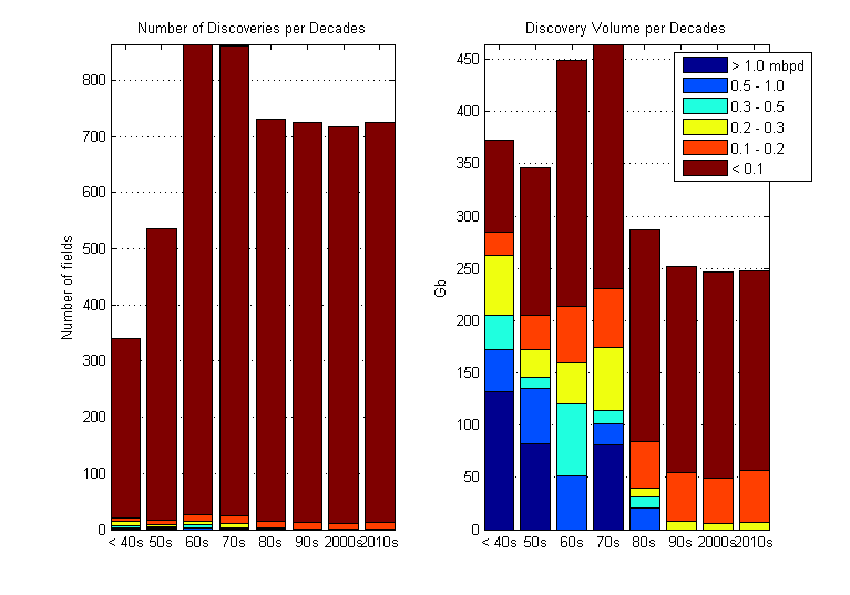
I finally found some info in Simmons's book in the appendix B (p. 374 and 375):
$this->bbcode_second_pass_code('', '
[i]volume and production in mb and mbpd[/i]
Field Size No of Tot.
(production vol.) fields Prod <1950 50s 60s 70s 80s 90s
1,000+ 4 8,000 2 1 0 1 0 0
500-1,000 10 5,900 2 3 3 1 1 0
300-500 12 4,100 3 1 6 1 1 0
200-300 29 6,450 8 4 6 9 1 1
100-200 61 7,900 5 8 13 13 11 11
0-100 4,000+ 36,200 ? ? ? ? ? ?
Total 4,061+ 38,550 ? ? ? ? ? ?
')
the last line is taken from Figure B.1 p. 374 but there are no information on the time of discovery distribution. The production figures are for 2000.
Last edited by khebab on Wed 05 Oct 2005, 19:38:40, edited 1 time in total.
______________________________________
http://GraphOilogy.blogspot.com
http://GraphOilogy.blogspot.com
- khebab
- Tar Sands
- Posts: 899
- Joined: Mon 27 Sep 2004, 03:00:00
- Location: Canada
Re: A Statistical Model for the Simulation of Oil Production
![]() by khebab » Tue 04 Oct 2005, 22:01:46
by khebab » Tue 04 Oct 2005, 22:01:46
Here the corresponding bar chart (without the small fields):

Figure 8
Figure 8
Last edited by khebab on Thu 06 Oct 2005, 21:28:51, edited 1 time in total.
______________________________________
http://GraphOilogy.blogspot.com
http://GraphOilogy.blogspot.com
- khebab
- Tar Sands
- Posts: 899
- Joined: Mon 27 Sep 2004, 03:00:00
- Location: Canada
Re: A Statistical Model for the Simulation of Oil Production
![]() by WebHubbleTelescope » Tue 04 Oct 2005, 23:56:53
by WebHubbleTelescope » Tue 04 Oct 2005, 23:56:53
$this->bbcode_second_pass_quote('EnergySpin', '')$this->bbcode_second_pass_quote('rockdoc123', 'E')nergySpin
I agree with your comment regarding the need to look at this with a stochastic view. I've actually played around with simpler models than Khebab used here...generally just for one or two pools. My assumptions are more general (assume peak production after 1 year ramp up...peak at 10% of URR...held for 2 - 5 years depending on field size and then declined at 10% /annum) but are what we normally use as first approximations. Usually I put in lognormal distributions for reserves and other assumptions regarding production/depletion. I've been using Crystal Ball in Excel but also have @Risk on my laptop. Pup55 sent me his Saudi depletion profile in excel format quite awhile ago and I have been meaning to fiddle around with that in Crystal Ball...unfortunately there are more things I would like to do than I have time for.
To my mind this whole discussion around Peak Oil could benefit greatly from discussing both reserves and production/depletion and demand from a stochastic viewpoint.
We all wished we had more time; PO is rather expensive hobby as far as time is concerned.
I did give Verhulst/logistic modelling a shot a while back in this forum and I was appaled. This is a nasty curve to fit data to; I'm not surprised that most predictions have been wrong. ....
I appreciate your take and expertise on data regression. But like Rockdoc, I have heartburn with the logistic model for more fundamental reasons. Why should it work at all for this class of behaviors? When did the strong non-linear component of the basic "predator/prey" get applied to oil depletion?
I have been playing around a lot with the stochastic formulation staying away from the non-linear terms, apart from the forcing function which corresponds to newly tapped discoveries.
Symmetric Triangular discovery window

Welch (upside down parabola) discovery window -- "logistic"-like

Khebab has got some curves with some of the same characteristics, but again, I just do not like the fact that we are solving the Verhulst equation to provide the parametric fits.
I have time to work this out some more. I have a post up where I list the posts I have done in the last few months.
http://mobjectivist.blogspot.com/2005/1 ... posts.html
Recently, I have tried to account for the oil shocks and even more recently have tried to understand the mathematical and physical underpinnings of the logistic curve model. Like I said, a bit frustrating that last bit. On the other hand, a stochastic model works brilliantly to account for oil shocks, i.e. the dips in the production curves.
-

WebHubbleTelescope - Tar Sands
- Posts: 950
- Joined: Thu 08 Jul 2004, 03:00:00


 .
.