[WebHubbleTelescope]

I tried out my macro model on USA lower-48 production using the same base parameters as I used for the global production fit:
http://mobjectivist.blogspot.com/2005/1 ... er-48.html



What's also interesting about the results, since it is a causal model, the fit would have been pretty much the same if attempted in the year 1957! In other words, no need to know the URR.

[EnergySpin]

WHT causal models can be used to estimate the URR .
One word of caution ... run the exercise with the data in 1957. It will give you an idea of how sensitive the procedure is in tracking the overall shape of the curve. Once you are past the peak ... the algorithm knows way too much. What is the URR that you got?
I did take a look into the North Sea profiles ... some of them are pretty atypical compared to the US profiles
ES

[doufus]

I don't want to rain on this parade. I have a great deal of respect for
modelling but it has enormous problems when applied to this domain.

Remember, modelling (despite claims to the contrary) can never
establish a causal chain. Even if the data fits perfectly there is alway
the chance that another, hidden constellation of variables is at work or that
another model with entirely different assumptions fits the data
equally as well. Which one is the "correct" one?

Modelling is tuff enough even when applied to valid and reliable
data. The data we have to work with here is neither.

I'm not suggesting you don't do it, but at the end of the day, apart
from having some fun, you may not have any greater certainty
about anything at all.

[EnergySpin]

$this->bbcode_second_pass_quote('doufus', 'I') don't want to rain on this parade. I have a great deal of respect for
modelling but it has enormous problems when applied to this domain.

Remember, modelling (despite claims to the contrary) can never
establish a causal chain. Even if the data fits perfectly there is alway
the chance that another, hidden constellation of variables is at work or that
another model with entirely different assumptions fits the data
equally as well. Which one is the "correct" one?

Modelling is tuff enough even when applied to valid and reliable
data. The data we have to work with here is neither.

I'm not suggesting you don't do it, but at the end of the day, apart
from having some fun, you may not have any greater certainty
about anything at all.

[WebHubbleTelescope]

$this->bbcode_second_pass_quote('EnergySpin', 'W')HT causal models can be used to estimate the URR .
One word of caution ... run the exercise with the data in 1957. It will give you an idea of how sensitive the procedure is in tracking the overall shape of the curve. Once you are past the peak ... the algorithm knows way too much. What is the URR that you got?
I did take a look into the North Sea profiles ... some of them are pretty atypical compared to the US profiles
ES

[WebHubbleTelescope]

$this->bbcode_second_pass_quote('doufus', 'R')emember, modelling (despite claims to the contrary) can never establish a causal chain.

[doufus]

$this->bbcode_second_pass_quote('WebHubbleTelescope', '')$this->bbcode_second_pass_quote('doufus', 'R')emember, modelling (despite claims to the contrary) can never establish a causal chain.

[Doly]

The testing of a model comes in the prediction. If it predicts well the behaviour of the system you are trying to model, it's a good model. If not, it isn't. We only have to wait to see if these models are any good.

[doufus]

$this->bbcode_second_pass_quote('EnergySpin', '')$this->bbcode_second_pass_quote('doufus', 'I') don't want to rain on this parade. I have a great deal of respect for
modelling but it has enormous problems when applied to this domain.

Remember, modelling (despite claims to the contrary) can never
establish a causal chain. Even if the data fits perfectly there is alway
the chance that another, hidden constellation of variables is at work or that
another model with entirely different assumptions fits the data
equally as well. Which one is the "correct" one?

Modelling is tuff enough even when applied to valid and reliable
data. The data we have to work with here is neither.

I'm not suggesting you don't do it, but at the end of the day, apart
from having some fun, you may not have any greater certainty
about anything at all.

[doufus]

$this->bbcode_second_pass_quote('Doly', 'T')he testing of a model comes in the prediction. If it predicts well the behaviour of the system you are trying to model, it's a good model. If not, it isn't. We only have to wait to see if these models are any good.

[WebHubbleTelescope]

$this->bbcode_second_pass_quote('doufus', 'O')r have we just created
an equation that fits a curve derived from zillions of processes- none
of which we know much about and none of which will be replicated in the
future.

[doufus]

$this->bbcode_second_pass_quote('WebHubbleTelescope', '')$this->bbcode_second_pass_quote('doufus', 'O')r have we just created
an equation that fits a curve derived from zillions of processes- none
of which we know much about and none of which will be replicated in the
future.

[SilentE]

Web,

is that discovery database backdated?

[khebab]

Here is my code in R language. It's my first experience with R so there are probably a lot of mistakes. In particular, the graphics sucks because plotting functions in R are quite complex!

The R software can be downloaded here:

http://www.r-project.org/

feel free to modify and improve it!

$this->bbcode_second_pass_code('', '####################################################################
##
## Script that simulates oil field discovery data and try to infer
## the total world production by adding individual logistic/Verhulst functions.
##
## see the thread http://www.peakoil.com/fortopic13463.html for more details
##
## Author: Khebab (October, 2005)
## version 1.0
##
####################################################################

rm(list=ls(all=TRUE)) # clean up
##
## Load matlab emulator package and gremisc (to install)
## in the menu bar: packages/install pacakage(s)
##
library(matlab)
library(gregmisc)
##
## Function SimulateDiscoveryData
##
## generates oilfield random deviates which have
## a pdf similar to the observed world discovery data
##
SimulateDiscoveryData <- function(mDiscoveryData, nNumberOfFields) {
nDecades= ncol(mDiscoveryData)-1;
vDiscoveryPdf <- colSums(mDiscoveryData[,2:(nDecades+1)]) / sum(sum(mDiscoveryData[,2:(nDecades+1)]))
vDiscoveryFieldCategoryPerDecades <- mDiscoveryData[,2:(nDecades+1)] / matrix(rep(as.vector(colSums(mDiscoveryData[,2:(nDecades+1)])), 6), nrow= 6, byrow= T)
vP <- 0.01:5000; # range od field output (in tbpd)
vLogNormalCDF <- plnorm(vP, sdlog= 4.2258) # lognormal distribution for the oilfield size distribution
vMin <- rev(c(plnorm(0.01, sdlog= 4.2258), plnorm(100.01, sdlog= 4.2258),
plnorm(200.01, sdlog= 4.2258), plnorm(300.01, sdlog= 4.2258), plnorm(500.01, sdlog= 4.2258), plnorm(1000.01, sdlog= 4.2258)))
vMax <- rev(c(plnorm(100, sdlog= 4.2258), plnorm(200, sdlog= 4.2258),
plnorm(300, sdlog= 4.2258), plnorm(500, sdlog= 4.2258), plnorm(1000, sdlog= 4.2258), plnorm(5000, sdlog= 4.2258)))
mRange <- cbind(vMin, vMax)
#
# Sampling of the discovery per decades pdf
#
vDiscoveryDecades <- sample(c(1:nDecades), nNumberOfFields, replace = T, prob= vDiscoveryPdf)
vDiscoveryDecades <- hist(vDiscoveryDecades, breaks= 0.5:(nDecades+0.5), plot= F)$counts
#vDiscoveryDecades <- matrix(floor(vDiscoveryPdf * nNumberOfFields), nrow= 1, ncol= nDecades)

#
# Sampling of the categories per decades pdf
#
mCategoryPerDecades <- matrix(0, nrow= 6, ncol= nDecades)
for (i in 1:nDecades) {
mCategoryPerDecades[,i] <- hist(sample(c(1:6), vDiscoveryDecades[i] , replace = T, prob= vDiscoveryFieldCategoryPerDecades[,i]), breaks= 0.5:(6+0.5), plot= F)$counts
#mCategoryPerDecades[,i] <- floor(vDiscoveryFieldCategoryPerDecades[,i] * vDiscoveryDecades[i])

}
#barplot(mCategoryPerDecades,xlab= "Decades", ylab= "Number of Fields", col=rainbow(20))
#title(main = "Simulated Number of oilfields in 2000", font.main = 3)
##
## importance sampling of the field size pdf according ot the pattern of discovery
## for each deacades
##
modifiedLogNormal <- function(x) vP[which(vLogNormalCDF >= x)[1]]

n <- 1;
mOilFieldsData <- matrix(0, nrow= nNumberOfFields, ncol= 7)
##
## For each discovery we randomly choose the oilfield parameters (year of discovery, meand field output, k, n)
##
for (d in 1:nDecades) {
for (c in 1:6) {
nEnd <- n + mCategoryPerDecades[c, d] - 1;
if (mCategoryPerDecades[c, d] > 0) {
mOilFieldsData[n:nEnd, 1] <- d
mOilFieldsData[n:nEnd, 3] <- c
mOilFieldsData[n:nEnd, 4] <- runif(mCategoryPerDecades[c,d], 0.05, 0.15);
mOilFieldsData[n:nEnd, 5] <- runif(mCategoryPerDecades[c,d], 0.2, 5.0);

if (d > 1) mOilFieldsData[n:nEnd, 2] <- runif(mCategoryPerDecades[c, d], (d-1) * 10 +1930, 10 * d + 1930)
else mOilFieldsData[n:nEnd, 2] <- runif(mCategoryPerDecades[c, d], 1900, 1940)
mOilFieldsData[n:nEnd, 6] <- apply(matrix(runif(mCategoryPerDecades[c, d], min= vMin[c], max= vMax[c]), nrow= 1, byrow= T), 2, modifiedLogNormal) * 365 / 1000000

mOilFieldsData[n:nEnd, 7] <- mOilFieldsData[n:nEnd, 6] / mOilFieldsData[n:nEnd, 4] * (mOilFieldsData[n:nEnd, 5] + 1)^(1/mOilFieldsData[n:nEnd, 5] + 1)
}
n <- n + mCategoryPerDecades[c, d];
}
}
# form the output
output <- data.frame(decades = mOilFieldsData[,1], year= mOilFieldsData[, 2], category = mOilFieldsData[,3],
fieldoutput= mOilFieldsData[,6], URR= mOilFieldsData[,7], k= mOilFieldsData[,4], n= mOilFieldsData[,4])
rm(mOilFieldsData)
output
}

##
## Generalized Verhulst function
##
Verhulst <- function(y, location, scale, area, n) {
temp= (2^n - 1) * exp((y - location) * scale)
output= scale * area / n * temp / (1 + temp)^(1/n+1)
output
}

Logistic <- function(y, location, scale, area) {
temp= tanh(0.5*(y - location) * scale)
output= 0.25 * area * scale * (1 - temp * temp)
output
}

####################################################################
##
## Main
##
####################################################################

#
# World oil production since 1901 up to 2005 (from BP) in Gb (all liquids)
#
temp <- scan()
2.0000000e-001 1.6740000e-001 1.8180000e-001 1.9490000e-001 2.1800000e-001 2.1510000e-001
2.1330000e-001 2.6420000e-001 2.8560000e-001 2.9870000e-001 3.2780000e-001 3.4440000e-001
3.5240000e-001 3.8530000e-001 4.0750000e-001 4.3200000e-001 4.5750000e-001 5.0290000e-001
5.0350000e-001 5.5590000e-001 6.8890000e-001 7.6600000e-001 8.5890000e-001 1.0157000e+000
1.0143000e+000 1.0679000e+000 1.0968000e+000 1.2630000e+000 1.3250000e+000 1.4860000e+000
1.4100000e+000 1.3730000e+000 1.3100000e+000 1.4420000e+000 1.5220000e+000 1.6540000e+000
1.7920000e+000 2.0390000e+000 1.9880000e+000 2.0860000e+000 2.1500000e+000 2.2210000e+000
2.0930000e+000 2.2570000e+000 2.5930000e+000 2.5950000e+000 2.7450000e+000 3.0220000e+000
3.4330000e+000 3.4040000e+000 3.8030000e+000 4.2830000e+000 4.5190000e+000 4.7980000e+000
5.0180000e+000 5.6260000e+000 6.1250000e+000 6.4390000e+000 6.6080000e+000 7.1340000e+000
7.6613500e+000 8.1942500e+000 8.8877500e+000 9.5374500e+000 1.0285700e+001 1.1070450e+001
1.2620000e+001 1.3550000e+001 1.4760000e+001 1.5930000e+001 1.7540000e+001 1.8560000e+001
1.9590000e+001 2.1340000e+001 2.1400000e+001 2.0380000e+001 2.2050000e+001 2.2890000e+001
2.3120000e+001 2.4110000e+001 2.2980000e+001 2.1730000e+001 2.0910000e+001 2.0660000e+001
2.1050000e+001 2.0980000e+001 2.2070000e+001 2.2190000e+001 2.3050000e+001 2.3380000e+001
2.3900000e+001 2.3830000e+001 2.4010000e+001 2.4110000e+001 2.4500000e+001 2.4860000e+001
2.5510000e+001 2.6340000e+001 2.6860000e+001 2.6400000e+001 2.7360000e+001 2.7310000e+001
2.7170000e+001 2.8120000e+001 2.9290000e+001 2.9830000e+001

vWorldProduction <- matrix(temp, ncol=1 , byrow= F)
vWorldProduction[106:200]= NA;
# Regular oil production from 1970-2005 (from ASPO)
vASPORegularOil <- matrix(c(15.9, 20.2, 20.8, 19.0, 21.0, 21.4, 23.12, 24.1), ncol= 8)

#
# Crude Oil prices (adjusted from inflation)
#
temp <- scan()
1.0350000e+001 1.9950000e+001 4.8530000e+001 9.7790000e+001 8.1670000e+001 4.8440000e+001
3.2680000e+001 5.1710000e+001 5.1850000e+001 5.7870000e+001 6.8710000e+001 5.7630000e+001
2.8970000e+001 1.9620000e+001 2.3320000e+001 4.5580000e+001 4.3090000e+001 2.3390000e+001
1.7500000e+001 1.8650000e+001 1.6890000e+001 1.5320000e+001 2.0330000e+001 1.7720000e+001
1.8560000e+001 1.4980000e+001 1.4130000e+001 1.8560000e+001 1.9830000e+001 1.8350000e+001
1.4130000e+001 1.1810000e+001 1.3500000e+001 1.8400000e+001 3.0970000e+001 2.6860000e+001
1.7990000e+001 2.0720000e+001 2.9360000e+001 2.7090000e+001 2.1860000e+001 1.7510000e+001
1.9830000e+001 1.8140000e+001 1.3080000e+001 1.5400000e+001 1.4640000e+001 1.5190000e+001
1.4770000e+001 1.2410000e+001 1.2410000e+001 1.4530000e+001 1.8220000e+001 1.5330000e+001
1.1990000e+001 1.9160000e+001 2.3140000e+001 2.5020000e+001 2.2110000e+001 2.9160000e+001
1.8400000e+001 1.8280000e+001 1.4950000e+001 1.5910000e+001 1.8240000e+001 2.0210000e+001
1.4240000e+001 1.2990000e+001 1.4100000e+001 1.3550000e+001 8.1200000e+000 1.2110000e+001
9.8300000e+000 1.4190000e+001 1.3430000e+001 1.4930000e+001 1.5600000e+001 1.5240000e+001
1.3950000e+001 1.3820000e+001 1.4700000e+001 1.3860000e+001 1.3180000e+001 1.3070000e+001
1.1080000e+001 1.0900000e+001 1.6150000e+001 1.5690000e+001 1.4180000e+001 1.3490000e+001
1.2500000e+001 1.2220000e+001 1.3690000e+001 1.3630000e+001 1.3680000e+001 1.3480000e+001
1.2810000e+001 1.3660000e+001 1.3550000e+001 1.2180000e+001 1.1420000e+001 1.1290000e+001
1.1150000e+001 1.1010000e+001 1.0830000e+001 1.0500000e+001 1.0230000e+001 9.8200000e+000
9.3200000e+000 8.7900000e+000 1.0500000e+001 1.1260000e+001 1.4050000e+001 4.4550000e+001
4.0660000e+001 4.1260000e+001 4.1620000e+001 3.9550000e+001 7.8460000e+001 8.2150000e+001
7.1470000e+001 6.2360000e+001 5.4730000e+001 5.1120000e+001 4.8460000e+001 2.4790000e+001
3.0640000e+001 2.3900000e+001 2.7750000e+001 3.4440000e+001 2.7840000e+001 2.6090000e+001
2.2330000e+001 2.0380000e+001 2.1310000e+001 2.5080000e+001 2.2740000e+001 1.5200000e+001
2.0710000e+001 3.1800000e+001 2.6440000e+001 2.6470000e+001 2.9610000e+001 3.8270000e+001
5.0000000e+001

vPrice <- matrix(temp, ncol=1 , byrow= F)

vPrice <- (vPrice - mean(vPrice)) / as.numeric(sqrt(var(vPrice)))
vPrice[length(vPrice)+1:200]= vPrice[length(vPrice)];

##
## Form a matrix of discovery data taken from Simmons
##
mDiscoveryData <-matrix(c(8.0,2,1,0,1,0,0,
5.9,2,3,3,1,1,0,
4.1,3,1,6,1,1,0,
6.45,8,4,6,9,1,1,
7.9,5,8,13,13,11,11,
36.2,666,666,666,666,666,666),nrow=6,byrow=T)
##
## For the small field pdf we have no data, onlt the approximate total number of field is
## known (4,000+). To simulate a pdf, we take the observed frequencies for the other field categories.
##
mDiscoveryData[6,2:7] <- colSums(mDiscoveryData[1:5,2:7]) / sum(sum(mDiscoveryData[1:5,2:7])) * 4000
##
## For the decades 200s and 2010s we replicate the same discovery pattern observed in the 90s but
## we reduce the amount of discovered small field by the same amount that was lost between the 80s and 90s
##
mDiscoveryData <- cbind(cbind(mDiscoveryData, mDiscoveryData[,7]), mDiscoveryData[,7])
#mDiscoveryData[6,8] <- mDiscoveryData[6,8] - (mDiscoveryData[6,6] - mDiscoveryData[6,7])
$mDiscoveryData[6,9] <- mDiscoveryData[6,8] - (mDiscoveryData[6,6] - mDiscoveryData[6,7])
mDiscoveryData <- cbind(mDiscoveryData, mDiscoveryData[,9])
$mDiscoveryData[6,10] <- mDiscoveryData[6,9] - (mDiscoveryData[6,6] - mDiscoveryData[6,7])
mDiscoveryData <- cbind(mDiscoveryData, mDiscoveryData[,10])
$mDiscoveryData[6,11] <- mDiscoveryData[6,10] - (mDiscoveryData[6,6] - mDiscoveryData[6,7])

dimnames(mDiscoveryData )<- list(c("1+ mbpd","0.5-1.0 mbpd","0.3-0.5 mbpd","0.2-0.3 mbpd","0.1-.2 mbpd","0-0.1 mbpd"),c("Total production (mbpd)","<40s","50s","60s","70s","80s","90s","2000s","2010s","2020s", "2030s"))

head(mDiscoveryData)
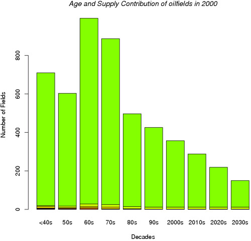
barplot(mDiscoveryData[,-c(1)],xlab= "Decades", ylab= "Number of Fields", col=rainbow(20))
title(main = "Age and Supply Contribution of oilfields in 2000", font.main = 3)

par(mfrow= c(1,1), pch="+", lty= 1)
#
# Total number of discovered field (affect the final URR)
#
nNumberOfFields <- 5500
#
# Number of runs
#
M <- 100
vProduction <- matrix(0, nrow= 200, ncol= M)
vResults <- array(NA, dim= c(200, 6, M))
vMeanResults <- matrix(NA, nrow= 200, ncol= 6)
mAnnualVolumeDiscovery <- matrix(0, nrow= 200, ncol= M)
vWeight <- matrix(0, nrow= 1, ncol= M)
#
# Main loop for the runs
#
vNumberOfFields= matrix(NA, nrow= M, ncol= 1)
nCentralNumberOfFields= sum(sum(mDiscoveryData[,2:ncol(mDiscoveryData)]));
for(m in 1:M) {
nNumberOfFields <- floor(runif(1,nCentralNumberOfFields - 1000, nCentralNumberOfFields + 1000))
vNumberOfFields[m] <- nNumberOfFields
# Simulate discovery data
tabOilFieldData <- SimulateDiscoveryData(mDiscoveryData, nNumberOfFields)
head(tabOilFieldData)
mOilFieldsCurves <- matrix(0, nrow= 200, ncol= nNumberOfFields)
#
# The production staring year is the discovery date randomly shifted by 6-25 years
#
tabOilFieldData$yearstart <- tabOilFieldData$year + runif(nNumberOfFields,6,25)
#tabOilFieldData$yearstart <- tabOilFieldData$yearstart - vPrice[floor(tabOilFieldData$yearstart)-1900];
categoryGroup <- factor(tabOilFieldData$category)
yearsFactor <- factor(1901:2100)
decadesGroup <- factor(tabOilFieldData$decades)

#volumes <- tapply(tabOilFieldData$URR, categoryGroup , sum)

#barplot(volumes ,xlab= "Category", ylab= "Gb", col=rainbow(20))
#volumes <- tapply(tabOilFieldData$URR, decadesGroup, sum)
#barplot(volumes ,xlab= "Decades", ylab= "Gb", col=rainbow(20))
#hist(tabOilFieldData$yearstart, seq(1901, 2050, 2), prob= F)
#lines(density(tabOilFieldData$yearstart, bw= 3))
#hist(tabOilFieldData$URR, seq(0, 120, 2), prob= F)
#lines(density(tabOilFieldData$URR, bw= 3))
idx <- 1:nNumberOfFields

r <- runif(nNumberOfFields, 0.1, 0.2)
#
# Compute each oilfield production curve
#
for(n in idx) {
#
# Compute a standard curve (logistic or Verhulst) with a unity area
#
#v <- Verhulst(1:400, 200, tabOilFieldData$k[n], 1, tabOilFieldData$n[n])
v <- Logistic(1:400, 200, tabOilFieldData$k[n], 1)
#
# truncate production at the beginning ( ensure causality)
#
idx <- find(v[1:200] < r[n] * max(v))
v[idx] <- 0
idx <- find(v > 0)
if (sum(v[idx]) > 0) {
#
# scale the curve in order to match the URR
#
v= v / sum(v[idx]) * tabOilFieldData$URR[n];
#v= v / mean(v[idx]) * tabOilFieldData$fieldoutput[n]; # alternative normalisation
vCumulative <- cumsum(v)
vCumulative[idx] <- (tabOilFieldData$URR[n] - vCumulative[idx]) / v[idx];
idx2 <- find(vCumulative < 5)
v[idx2] <- 0
#
# Shift the curve at the staring year position
#
nLength= 201 - floor(tabOilFieldData$yearstart[n]-1900);
mOilFieldsCurves[floor(tabOilFieldData$yearstart[n]-1900):200,n] <- v[idx[1]:(idx[1]+nLength-1)]

}
}

vTotalProduction <- rowSums(mOilFieldsCurves)
#
# The average curve can use a weighted mean
#
vWeight[m] <- 1.0
#vWeight[m] <- 1/mean((vTotalProduction[c(1:60, 82:105)] - vWorldProduction[c(1:60, 82:105)])^2)
vWeight[m] <- 1/mean(c((vTotalProduction[1:60] - vWorldProduction[1:60])^2, (vASPORegularOil[4:8] - vTotalProduction[seq(85, 105, 5)])^2))
vProduction[,m] <- vTotalProduction * vWeight[m]
fSumWeight <- sum(vWeight[1:m]);
tmp <- split(vProduction[,1:m] / fSumWeight, yearsFactor)
means <- sapply(tmp, mean) * m
stdev <- sqrt(sapply(tmp, var))
n <- sapply(tmp,length)
ciw <- stdev #qt(0.975, n) * stdev / sqrt(n)
#
# Compute production curves by category
#
for(n in 1:6) {
idx <- find(tabOilFieldData$category == n);
if (length(idx) > 1) vResults[,n,m] <- rowSums(mOilFieldsCurves[,idx] * vWeight[m])
else if (length(idx) > 0) vResults[,n,m] <- mOilFieldsCurves[,idx] * vWeight[m]
tmp <- split(vResults[,n,1:m] / fSumWeight, yearsFactor)
vMeanResults[,n] <- sapply(tmp, mean) * m
}
#vAnnualDiscovery <- tapply(tabOilFieldData$URR, factor(floor(tabOilFieldData$yearstart)), length)
#vAnnualVolumeDiscovery <- tapply(tabOilFieldData$URR, factor(floor(tabOilFieldData$yearstart)), mean)
#mAnnualVolumeDiscovery[,m] <- vAnnualVolumeDiscovery * vAnnualDiscovery * vWeight[m]
#vMeanVolumeDiscovery <- rowSums(mAnnualVolumeDiscovery) / fSumWeight
vTemp <- matrix(NA, nrow= 200, ncol= 1, , byrow= F)
#vTemp[1:69] <- vWorldProduction[1:69]
vTemp[seq(70, 105, 5)] <- vASPORegularOil
matplot(x= yearsFactor, y= cbind(vMeanResults, cbind(vTotalProduction, vWorldProduction)), pch = 1:4, type = "l", add= F, ylab= "Gb/year", xlab= "")
lines(x= seq(1970, 2005, 5), y= vASPORegularOil, add= T, type= "l", col= 2)
text(x= 2070,y= means[130], "Total production (Excl. Synth. Oil, NGL)",col= 1,cex=.7);
text(x= 2020,y= vMeanResults[120,1], "Cat. 1",col= 1,cex=.7);
text(x= 2020,y= vMeanResults[120,2], "Cat. 2",col= 1,cex=.7);
text(x= 2025,y= vMeanResults[120,3], "Cat. 3",col= 1,cex=.7);
text(x= 2025,y= vMeanResults[120,4], "Cat. 4",col= 1,cex=.7);
text(x= 2050,y= vMeanResults[150,5], "Cat. 5",col= 1,cex=.7);
text(x= 2050,y= vMeanResults[150,6], "Cat. 6",col= 1,cex=.7);
text(x= 1970,y= vWorldProduction[104], "Observed Production (All liquids)",col= 2,cex=.7);
text(x= 1925, y= 29, sprintf("Iter= %d No of Fields= %d", m, nNumberOfFields), col= 2, cex= .9)
text(x= 1915, y= 25, sprintf("URR= %6.3f Gb", sum(means)), col= 1, cex= .8)
text(x= 1915, y= 24, sprintf("PO= %6.3f", 1900 + which.max(means)), col= 1, cex= .8)
text(x= 1915, y= 23, sprintf("#Fields= %6.3f",sum(t(vWeight) * vNumberOfFields, na.rm= T) / sum(sum(vWeight, na.rm= T))), col= 1, cex= .8)
plotCI(x=1901:2100, y=means, uiw=ciw, col="black", barcol="blue", add= T, ylab= "Gb/year")

}
lines(x=c(1901,2100), y=c(24.1,24.1), lty= 4)
text(x= 2075, y= 26, "ASPO estimate (24.1 Gb)", cex= 0.6)
')

{edit: 10/11/2005 correction of a few bugs}

[khebab]

Two results of simulation using the code above with two different scenarios for future discoveries.

Middle case:
Same amount of new discoveries fot the 90s up to the 2030s.



The full red line is the ASPO estimate for regular oil whereas the dashed red line is the all liquids oil production from BP. The horizontal dashed line is the ASPO estimate for the regular oil peak (24.1 Gb)

Low case:
The amount of new discoveries (small fields) diminishes gradually from the 80s



Both give the same estiamte for the regular oil peak date (2006). The estimated URR is around 2,200 Gb. The middle case scenario produces a bumpier curve post PO due to a larger production plateau from small fields (Category 6 fields). Even if we keep the same rate of discoveries of the 90s , it seems that the PO date won't be push back.

[WebHubbleTelescope]

Whenever I see a plot of the logistic curve, I always like to see the expression with values for the coefficients next to it. I believe that this consists of an overall scaling parameter, an exponential factor, and a time shift on the exponential for the simplest version.

[khebab]

$this->bbcode_second_pass_quote('WebHubbleTelescope', 'W')henever I see a plot of the logistic curve, I always like to see the expression with values for the coefficients next to it. I believe that this consists of an overall scaling parameter, an exponential factor, and a time shift on the exponential for the simplest version.

[SilentE]

$this->bbcode_second_pass_quote('khebab', ' ')Even if we keep the same rate of discoveries of the 90s , it seems that the PO date won't be push back.

[Taskforce_Unity]

Your assumption is not correct SilentE. At the moment the average life after discovery when an oil field comes on-stream is approximately 4-6 years. Some oil fields come on-stream 2 years after they have been discovered!

[khebab]

$this->bbcode_second_pass_quote('SilentE', 'T')hat's an artifact produced by your model assumptions. The lag between discovery and production means that the production curve for 2000-2010 was 99.99% determined by discoveries before 2000. Thus, changing discoveries after 2000 should have no discernible effect on a peak of 2006. Eyeballing the two curves, the differences only appear on the backslope of the curve, a few decades hence.