Deepwater GOM: Reserves versus Production – Part 2: Atlantis, Mad Dog & Eugene Island

In the deepwater GOM, BP (in red) has the highest number of discoveries, as shown in this graph from PFC (R.West 2011), particularly with Atlantis and Mad Dog. Shell (in blue) is the second discoverer by number. The cumulative oil and gas discovery displays a typical S curve, but where is the asymptote?

Figure 29: Deepwater (>1000 ft) cumulative discovery from Chevron.

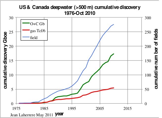
The cumulative deepwater (>500 m) discovery for the US and Canada by the Fall of 2010 was 18 Gb for oil and 30 Tcf for gas.

Figure 30: US and Canada deepwater (>500 m) cumulative discovery.

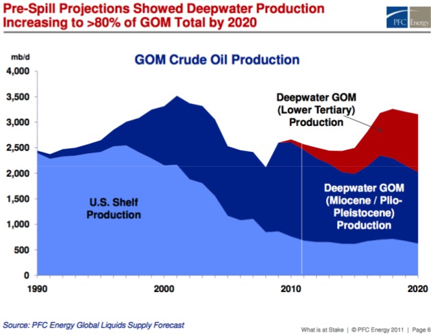
PFC forecasts GOM production to peak again in 2018 due to the Lower Tertiary plays discovered in recent years.

Figure 31: GOM crude oil production from 1990 to 2020 according to PFC.

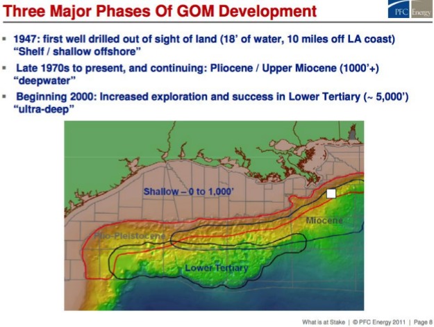
The following map shows the three phases of GOM exploration:

• 1947: shelf-shallow offshore
• late 1990s: Pliocene/Upper Miocene deepwater >1000 ft
• beginning 2000: Lower Tertiary ultra deep >5000 ft

Figure 32: Three major phases of GOM development from PFC.

Deepwater reserves (EUR) and oil-in-place (OOIP) are reported by Joseph Lach, Vice President of Reservoir Management in a document titled “Final Report to IOR for Deepwater Gulf of Mexico” published on 15 December 2010.

Figure 33a: Mature fields (1979-1999) deepwater EUR and OOIP from Lach.

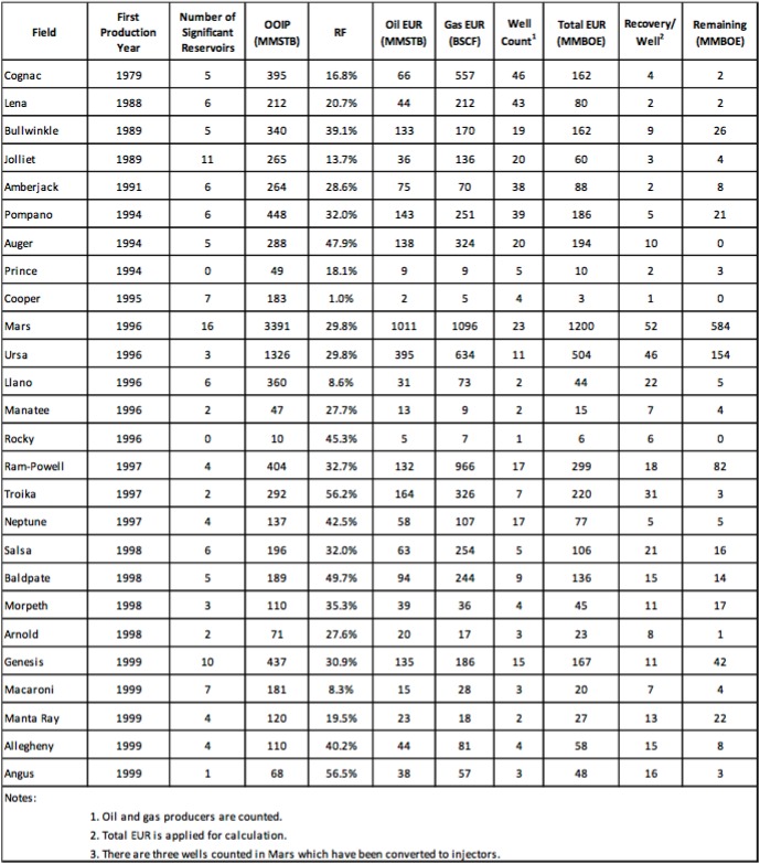Figure 33b: new oil fields (2000-2009) EUR from Lach.

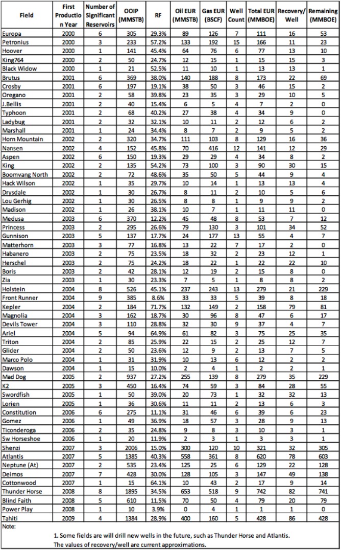The three significant digits on the recovery factor make me wonder about the understanding of the author on the accuracy of such estimates! OOIP are uncertain figures even at the end of field lifetime; moreover, the accuracy of recovery factors (RF) is about 10%, meaning that only the first digit can be considered as reliable: this is the reason why RF are often reported as rounded (e.g. 30%) or as fraction (e.g. one third).

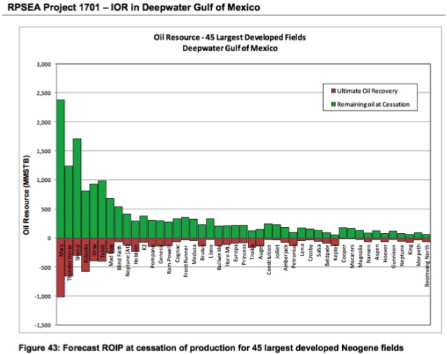
The 45 largest developed fields in the deepwater GOM are reported in a graph also in this document by Lach, showing the ultimate and remaining oil. This graph includes: Mars, Thunder Horse, Shenzi, Atlantis, Ursa, Tahiti and Mad Dog.

Figure 34: GOM deepwater: 45 largest oilfields from Lach.

After Thunder Horse and Mars/Ursa, let’s now study other large fields, starting with Atlantis as shown in the next map, operated by BP.

Figure 35: map of the fields developed by BP in the GOM.

Atlantis

The Atlantis field (also known as Green Canyon 743) includes in fact the Green Canyon blocks 699, 700, 742, 743, and 744, being located in the Central Gulf of Mexico about 190 miles south of New Orleans, Louisiana. BP and BHP Billiton jointly acquired leases on these blocks under OCS Sale 152 (held on May 10, 1995). BHP retains a 44% working interest in the project with BP being the designated operator. The oil field was discovered in 1998 by the Ocean America semi-submersible, mobile drilling rig operating in a water depth of 1870 metres (6140 ft). The Atlantis platform began production from two wells in October 2007. The Atlantis North Flank began production in July 2009. By 2010, there were twelve wells in production. Twenty wells were originally planned, including 16 producers and four water injection wells.

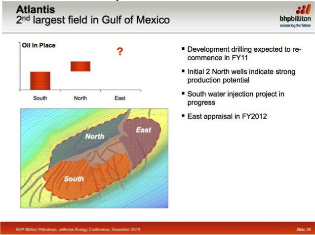
Atlantis is a structure with different compartments. New development will resume in 2011 and in 2012 with the appraisal of the eastern compartment. BHP is presenting more data on Atlantis than BP, the following graphs are taken from a presentation by Michael Yagger to the 2010 Jefferies Energy Conference .

Figure 36: map of Atlantis with its different compartments from BHP.

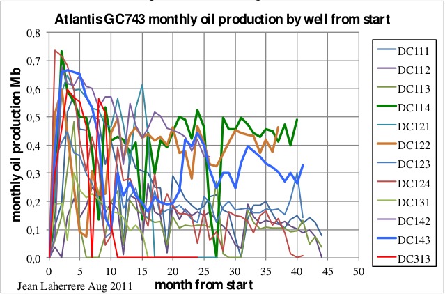
Up to May of 2011 the 12 producing wells display different behaviours in a plot of monthly production from the project start: some decrease, others like DC114 or DC122 do not. In addition to these, well DC102 did not produce anything.

Figure 37: Individual well oil production in the Atlantis field from production start.

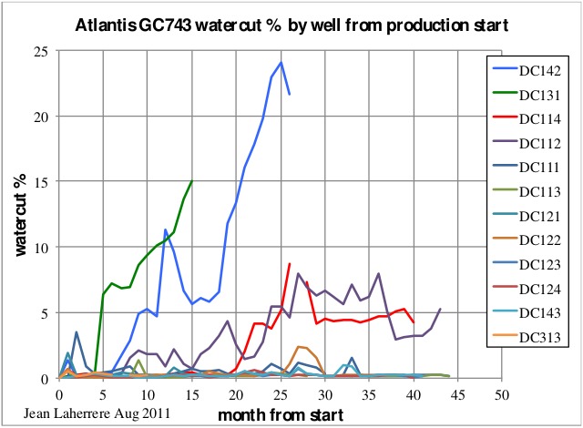
The watercut of those 12 wells behaves also quite differently: DC142 increases to 24% after 25 months; DC131 to 15% after 15 months; DC114 is stable at 5% after 40 months; DC112 went up and down and is now at 5% after 43 months; all other wells have less than 2%. Such low watercut is surprising when looking at the map presented by BHP that shows many faults.

Figure 38: Atlantis individual well watercut from production start.

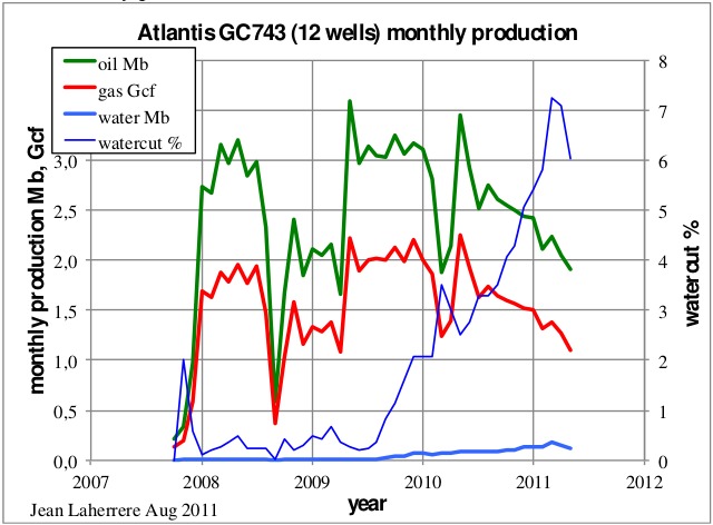
The total monthly production is erratic, but with a decline for oil since May of 2010. The total watercut started increasing sharply from the middle of 2009 but it is still only 7%, which is small when compared to the world average of 75%.

Figure 39: Atlantis monthly production.

The monthly oil production shows a decline of 2.5% per month since 2010, while the average daily production per well peaked at 18000 b/d in 2008, declined sharply that year and since the middle of 2009 is yielding a slower decline rate, around 2% per month.

Figure 40: Atlantis monthly and daily average per well oil production.

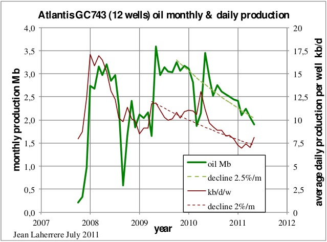Again, this trend refers to present wells, any new drilling will change the trend.

The following graph shows total monthly production versus cumulative production, from which it is hard to extrapolate lacking the plan for future drilling. BP has been very slow to resume drilling after the Macondo blowout when compared to other operators: for the first half of 2011, Shell had 16 drilling permits approved, Chevron had 23, BHP had 15, Exxon has had 11 and BP had none.

Figure 41: Atlantis oil decline.

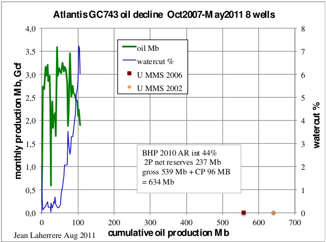MMS (now BOEMRE) has estimated the initial reserves in Atlantis at 641 Mb at the end of 2002, but 559 Mb at the end of 2006. BHP in their annual report for 2010 stated their net 2P oil reserves at 237 Mb (from a gross estimate of 539 Mb with a 44% factor for 2P). Adding to this the cumulative production at the end of 2010 of 96 Mb, the initial reserves sum up to 634 Mb. Lach (2010) has an estimated EUR at 558 Mb.

The oil decline can only be extrapolated when all the compartments are drilled and at this time the eastern compartment seems still yet to be drilled. It is thus impossible to say if Atlantis will be a giant oilfield (500 Mb).

Mad Dog

The Mad Dog field, discovered in 1998, is located in the Western Atwater Foldbelt, approximately 190 miles south of New Orleans, USA and is listed by the MMS as GC826. The field is operated by BP, which has a 60.5% share, the remaining stakes belong to BHP Billiton (23.9%) and Chevron (15.6%). The drilling unit is located in 5000 ft to 7000 ft of water in Green Canyon blocks 825, 826 and 782, about 150 miles southwest of Venice, Louisiana. The gross estimated reserves are in the range of 200 to 450 million barrels of oil equivalent. The facility can produce around 80,000 b/d of oil and 60 Mcf/d of natural gas.

A well extending towards the southern region of the field known as “Mad Dog Southwest Ridge” was drilled in March of 2005 and appraised in July of 2009. Drilling results identified around 280 ft of hydrocarbons of Miocene sand and an oil column of over 2200 ft. In 2008 another well, known as A-7, extending towards the western region of the field, identified a hydrocarbon column over 2500 ft with 275 ft of net pay. This field is presently being developed by 12 wells.

The Mississippi fan fold belt is characterised by basinward-verging anticlines and associated thrust faults. Mad Dog is one of a number of discoveries occurring in the western portion of the fold belt, where shallow salt tongues have flown over some of the folds, making seismic imaging difficult.

A seismic profile was shown by Hudec et al (AAPG 2006) as a trap below a salt canopy.

Figure 42: Mad Dog seismic profile.

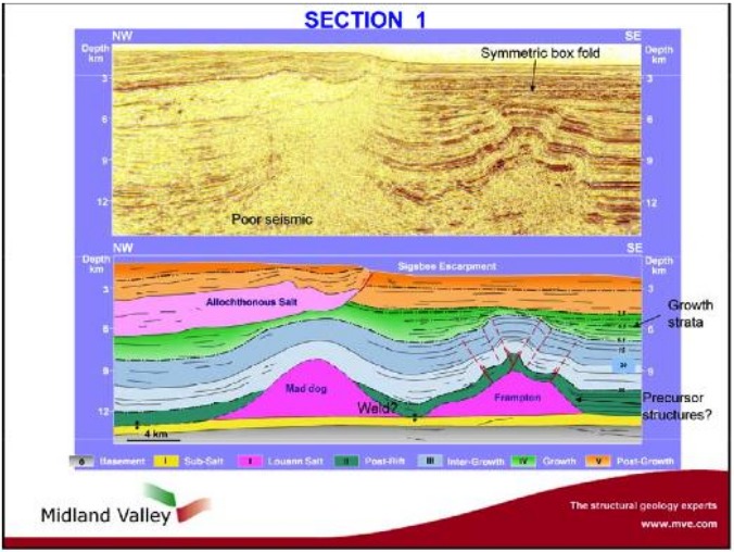
A simplified interpretation was presented by Grando et al (AAPG 2009) as an anticlinal trap above a salt diapir (pink) and below allochthonous salt. The seismic signal below the salt is described as poor!

Figure 43: Mad Dog interpretation by Grando et al.

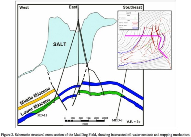
A detailed interpretation of the structure (profile and map) was presented by Dias et al (AAPG 2009). On the profile, the structure is faulted with a wet compartment (graben) in the middle.

Figure 44: Mad Dog cross section from Dias et al.

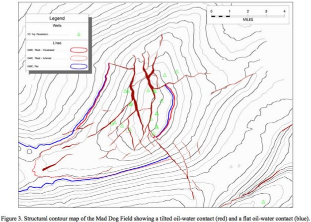
The locations of 14 wells are mapped as tilted (red) and flat (blue) oil-water contacts.

Figure 45: Mad Dog map from Dias et al.

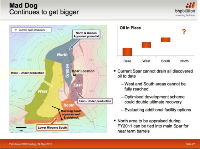
The presentation by Michael Yagger to the 2010 Jefferies Energy Conference shows the potential increase and indicates that the South and West areas of the field are out of reach of the platform presently being used, Spar. The North section of the field is planned to be appraised still in 2011.

Figure 46: Mad Dog map from BHP.

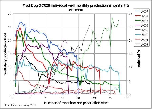
Contrary to Atlantis, the MMS monthly oil production data per well (available for 8 wells) shows decreases in parallel from production start. In some cases the watercut is already over 30% after 50 to 60 months of production, but for the majority of the wells it has remained very low.

Figure 47: Mad Dog individual well monthly oil production and watercut.

The total monthly production for oil, gas and water with the total number of production days shows an increase from 2005 to the peak at the beginning of 2009. Discounting the quasi-annual stoppages for maintenance, the decline is almost symmetrical to the rise.

Figure 48: Mad Dog monthly production from 8 wells and number of production days.

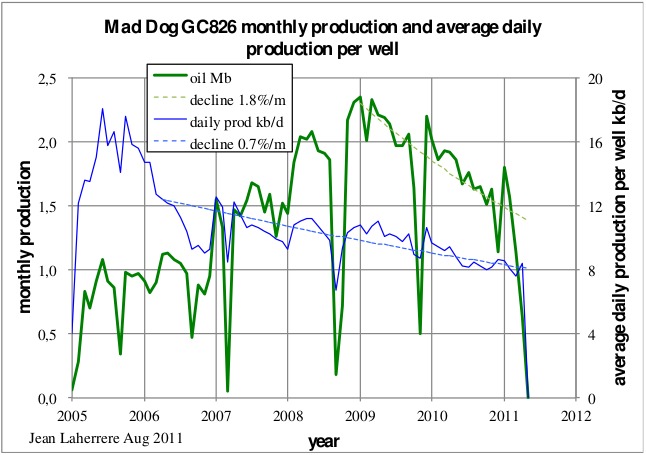
Following is a plot of monthly oil production, which peaked in January of 2009 at 2.3 Mb/m, together with the average daily production per well, which peaked at 17,000 b/d by the middle of 2005. Monthly oil total production declines at about 1.8% per month; when the average daily production per well declines at only 0.7% per month.

Figure 49: Mad Dog monthly oil production and average daily production per well.

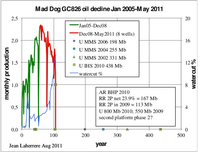
The next graph shows monthly oil production versus the cumulative production, with the various ultimate estimates. It is amazing to see MMS estimates decreasing from 2002 at 331 Mb to 2006 at 198 Mb, while BHP claims initial reserves around 800 Mb (167 Mb net + 101 Mb cum prod) in 2010, with a sharp increase from their 2009 estimate of 550 Mb (113 Mb net + 80 Mb cum prod). In 2010 IHS estimated the ultimate to be 438 Mb (up from 255 Mb in 2004, 195 Mb in 2003 and 193 Mb in 1999). Also in 2010, Lach reported the ultimate at 255 Mb.

It will be interesting to see the next BOEMRE oil and gas reserves estimate for the of end 2007. Past production cannot yet tell which ultimate is right, because the full filed structure is not yet completely appraised!

Figure 50: Mad Dog oil decline.

Eugene Island 330 (EI330)

Back in December of 2003, I gave a presentation “How to estimate future oil supply and oil demand?” at Copenhagen to the International Conference on Oil Demand, Production and Costs – Prospects for the Future, organized by the Danish Technology Council and the Danish Society of Engineers. In it I studied the oil depletion at the end of 2000 of several oil fields in the GOM: EI330, WD030 and SP027. It is interesting to update those three fields.

This Eugene Island field is famous because of a 1999 Wall Street Journal (WSJ) article that started a controversy about its oil depletion rate because of refilling from a deeper source. Astronomer T. Gold claimed this was proof of an abiogenic nature to oil, originating in the Earth’s mantle, and that EI330 also explained the large increase (300 Gb) in OPEC reserves during the second half of the 1980s (due in fact to their fight on quotas).

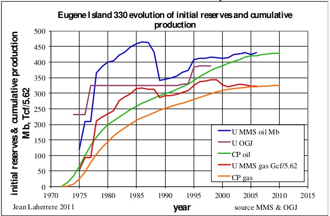
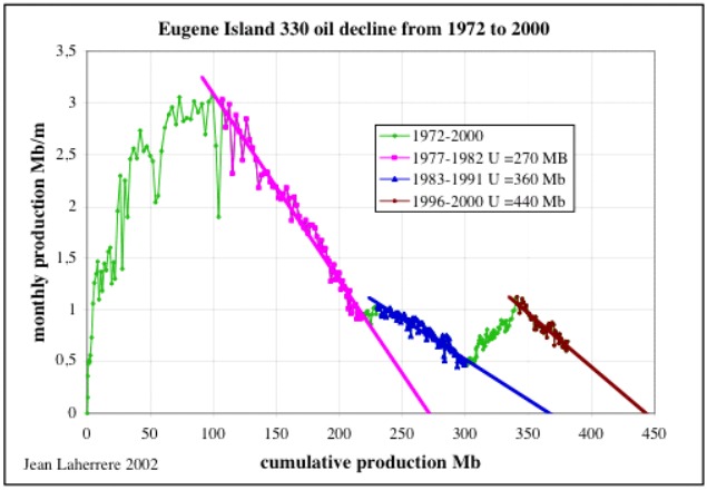
EI330 was discovered in December of 1971 by Pennzoil and Shell in shallow water (247 ft) and production started in September of the following year. In 1983, up to nine platforms were installed. Production peaked around 100,000 b/d in 1976 for a short period of time; during that year EI330 was the largest offshore oil producer with 31 Mb. But it declined sharply afterwards, at 2% per month up to 1983; this decline then slowed to less than 1% per month up to 1992, when the production started to increase to a new peak in 1996, when the mystery of EI330 made it to the newspapers. The WSJ was wrong by stating that “the reserves have rocketed to more than 400 Mb from 60 Mb”. Initial reserves estimates by the MMS were 120 Mb in 1975, 460 Mb in 1986, 350 Mb in 1989 and 410 Mb in 1996; it is difficult to see a rocket – it is behaving more like a drunk fly.

The following graph shows this evolution for oil and gas ultimate reserves estimated by the MMS and the OGJ, plus cumulative production. No mystery, except that the MMS reserve estimate was chaotic!

Figure 51: EI330 evolution of initial reserves and cumulative production.

The explanation of the mystery on this production increase is geological. The EI330 trap is against one of the largest faults in the GOM. After considerable production, the pressure, which is typically huge in these Plio-Pleistocene reservoirs, dropped to a point where it allowed refilling from the source-rock, with which these reservoirs are in direct communication. The migration between source-rock and the trap usually takes a long time: here the assumed refilling starting in 1992 was quick (few years) in geological time.

In a presentation entitled “Oil and gas: what future?” delivered at Groningen in the 21st of November of 2006 I wrote:

There is another example of exceptional positive reserve growth, which is Eugene Island 330 in the Gulf of Mexico. The largest fault in the area called the Red Fault (studied on the web by several universities) allows the reservoir to be directly in communication to the source rock and when the pressure dropped the reservoir was fairly quickly recharged by the source-rock. In 1999, Wall Street Journal (Cooper) stated from this example that oil was coming from the mantle, making oil renewable and almost unlimited.

Figure 11: Oil decline of Eugene Island 330 (US Gulf of Mexico) 1972-2003.

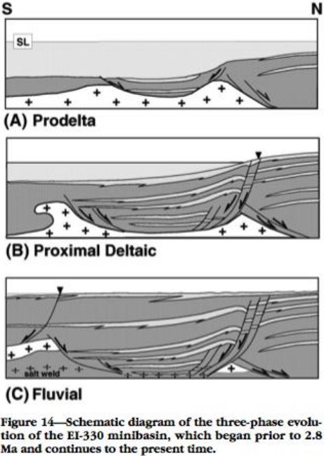
An MSc thesis by B.B. Stump (Pennsylvania State University, December 1998) studied over pressures in some EO330 reservoirs. Laurel L. Alexander and Peter B. Flemings in “Geologic Evolution of a Pliocene–Pleistocene Salt-Withdrawal Minibasin: Eugene Island Block 330, Offshore Louisiana” (AAPG Dec 1995 v79 n°12 p1737-1756) explain the formation of the EI330 reservoirs and respective trap, with this large fault.

Figure 52: EI330 schematic diagram on the evolution of the three geological phases.

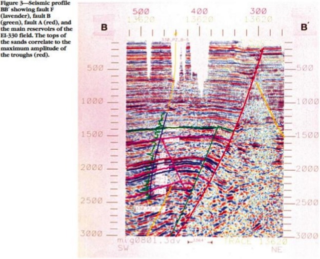
In the AAPG of March 1998, the same L.L. Alexander displays a seismic profile with the A fault (in red), which goes from the deep towards the surface.

Figure 53: EI330 seismic profile with the A fault (in red).

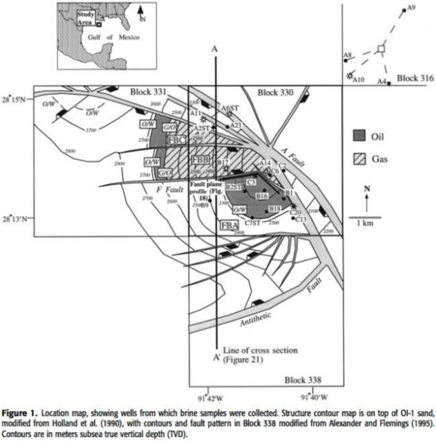
The following map is from “Reservoir fluids and their migration into the South Eugene Island Block 330 reservoirs, offshore Louisiana” by Steven Losh et al. EI330 is also called South Eugene Island block 330 (SEI330).

Figure 54: EI330 structure map on sand OI-1.

In 2004, EI330 was studied to be used for CO2 sequestration (M.D.Zoback et al).

Figure 55: GOM infrastructure with EI330 (SEI330) in 2000 (red = oil pipeline, green = gas pipeline).

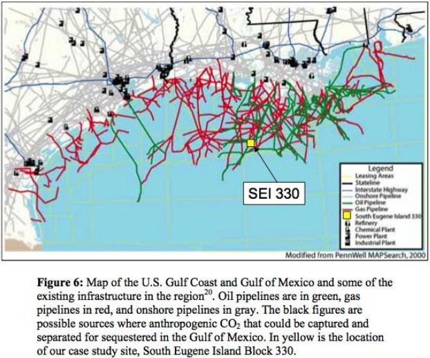The following diagram shows the pressure of some reservoirs between the overburden and hydrostatic pressure.

Figure 56: EI330 pressure diagram.

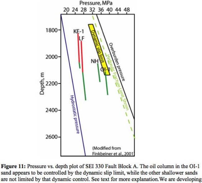This explains that when a reservoir is depleted, lowering the pressure and the resulting lack of pressure, it attracts the migration and recharge of oil through the A fault from the deep source–rock to the reservoir. But the present data shows that the recharge was limited.

The compilation of every GOM field production is given by MMS in their estimate of oil and gas reserves, but the last report is dated of 2009, reporting up to the end of 2006. As mentioned in part 1, I went to the BOEMRE site where there are several (3) reports by unit or per lease and used the shorter one (per unit) which reports only monthly oil, gas and water production by field. But for EI330 I got for 2006 unit monthly oil production ten times less than from the reserves data. To find the source of this discrepancy I went to the production per lease, which details the production broken down into crude oil and condensate (also gas-well gas and casing gas) and I found that the per unit data reports only a part of the data. For example, for 201001, lease G02115 the total for the month of January:

• unit file in page 837 reports only one well (B015) with 149 b for oil and 0 b for water;
• lease file PBOGORAL in page 1834 reports 30 wells with a total of 15 915 b for oil, 145 907 kcf for gas and 90 443 b for water;
• production file PBP9152A in page 1243 reports 20 wells with 15 766 b for oil, 149 b for condensate, 129 268 kcf for gas-well gas, 16 639 kcf for casing gas and 90 443 b for water.

The unit file is incomplete and provides wrong data. I was obliged to go to the OGORA file, which is much more voluminous (5031 pages for 2006 in pdf).

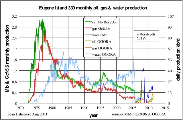
The monthly oil, gas, and water production displays the two oil peaks in 1976 and 1996, with a collapse in 2005 with Katrina, followed by a recovery!

Figure 57: EI330 monthly production.

The monthly oil production versus cumulative production shows that the field is close to depletion and that the initial reserves estimated by the MMS in 2006 could be few MB too short, but their 1986 estimate is likely too high.

Figure 58: EI330 oil decline, watercut and ultimates.

The more recent data (from OGORA) also allows to plot the average daily production per well from 2007 up to now; the decline is from 200 b/d/w in 2007 to about 100 b/d/w today, which is circa 2%/month.

Figure 59: EI330 average daily production per well.

This field will likely be abandoned in the next few years.

The Oil Drum