Since 2006, I’ve been tracking a set of oil production forecasts and trying to see how they performed over time. Comparing oil supply forecasts is not an easy task because of the many different assumptions, baselines, and fuel categories included. Also, most of them deal with production capacity which is almost impossible to track as we can only observe delivered supply. Since the 80s, oil production has pretty much followed population growth; using a ratio value of 4 barrels/person/year, one can accurately predict supply level for crude oil plus NGL (C+C+NGL) with an accuracy of +/- 2 Mbpd. This naive model will constitute my Null hypothesis (or model M0) that supply is not being constrained. Consequently, what could constitute a kind of “peak oil signal” would be a statistically significant deviation (I would be happy with only 2 sigmas) from the population based model M0. As we can see on the figure below, crude oil and NGL has not deviated significantly from M0. However, if we remove the contribution from Canadian tar sands and tight oil (shale oil), we can see that the deviation starts to be statistically significant.

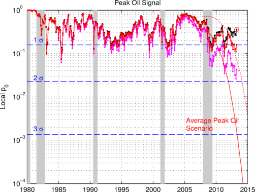
Hypothetical peak oil signal for C+C+NGL. Light gray bands indicate recessions. The dotted black curve is for C+C+NGL, the dotted red curve excludes tight oil and the magenta curve excludes Canadian tar sands. The continuous red line is the statistical significance corresponding to  the average peak oil scenario.

Notations:

• mbpd= Million of barrels per day

• Gb= Billion of barrels (10⁹)

• Tb= Trillion of barrels (10¹²)
• NGPL= Natural Gas Plant Liquids
• CO=C+C= Crude Oil + Lease Condensate
• NGL= Natural Gas Liquids (lease condensate + NGPL)
• URR= Ultimate Recoverable Resource

EIA Last Update (April)

Data sources for the production numbers:

• Production data from BP Statistical Review of World Energy (Crude oil + NGL).
• EIA data (monthly and annual productions up to March 2009) for crude oil and lease condensate (noted CO) on which I added the NGPL production (noted CO+NGL).

For the last two years, production has grown significantly and production records have been broken on a monthly basis, however, one can see that “conventional” crude oil is on a slightly downward plateau since 2005.

Fig 1.- World production (EIA data). Blue lines and pentagrams are indicating monthly maximum. Monthly data for CO from the EIA. Annual data for NGPL and Other Liquids from 1980 to 2001 have been upsampled to get monthly estimates. 

Business as Usual

• EIA’s International Energy Outlook 2006, reference case (Table E4, World Oil Production by Region and Country, Reference Case).
• IEA total liquid demand forecast for 2006 and 2007 (Table1.xls).
• IEA World Energy Outlook 2008, see post here for details.
• IEA World Energy Outlook 2006: forecasts for All liquids, CO+NGL and Crude Oil (Table 3.2, p. 94).
• IEA World Energy Outlook 2005: forecast for All liquids (Table 3.5).
• IEA World Energy Outlook 2004: forecast for All liquids (Table 2.4).
• A simple demographic model based on the observation that the oil produced per capita has been roughly constant for the last 26 years around 4.45 barrels/capita/year (Crude Oil + NGL). The world population forecast employed is the UN 2004 Revision Population Database (medium variant).
• CERA forecasts for conventional oil (Crude Oil + Condensate?) and all liquids, believed to be productive capacities (i.e. actual production + spare capacity). The numbers have been derived from Figure 1 in Dave’s response to CERA.

Fig 2.- Production forecasts assuming no visible peak.

PeakOilers: Bottom-Up Analysis

• Chris Skrebowski’s megaprojects database (see discussion here).
• The ASPO forecast from April newsletter (#76): I took the production numbers for 2000, 2005, 2010, 2015 and 2050 and then interpolated the data (spline) for the missing years. I added the previous forecast issued one year and two years ago (newsletter #58 and #46 respectively).
• Rembrandt H. E. M. Koppelaar (Oil Supply Analysis 2006 – 2007): “Between 2006 and 2010 nearly 25 mbpd of new production is expected to come on-stream leading to a production (all liquids) level of 93-94 mbpd (91 mbpd for CO+NGL) in 2010 with the incorporation of a decline rate of 4% over present day production”.
• Koppelaar Oil Production Outlook 2005-2040 – Foundation Peak Oil Netherlands (November 2005 Edition).
• The WOCAP model from Samsam Bakhtiari (2003). The forecast is for crude oil plus NGL.
• Forecast by Michael Smith (was at the Energy Institute, now works for EnergyFiles) for CO+NGL, the data have been taken from this chart in this presentation (The Future for Global Oil Supply (1641Kb), November 2006.).
• PhD thesis of Frederik Robelius (2007):  Giant Oil Fields – The Highway to Oil: Giant Oil Fields and their Importance for Future Oil Production. The forecasts (low and high) are derived from this chart.
• Forecast by TOD’s contributor Ace, details can be found in this post.
• The forecast by Duncan and Youngquist  made in 1999, see also this post by Euan Mearns.

Fig 3.- Forecasts by PeakOilers based on bottom-up methodologies. 

PeakOilers: Curve Fitting

The following results are based on a linear or non-linear fit of a parametric curve (most often a Logistic curve) directly on the observed production profile:

• Professor Kenneth S. Deffeyes forecast (Beyond Oil: The View From Hubbert’s Peak): Logistic curve fit applied on crude oil only (plus condensate and probably excluding tar sand production) with URR= 2013 Gb and peak date around November 24th, 2005.
• Jean Lahèrrere (2005): Peak oil and other peaks, presentation to the CERN meeting, 2005.
• Jean Lahèrrere (2006): When will oil production decline significantly? European Geosciences Union, Vienna, 2006.
• Logistic curves derived from the application of Hubbert Linearization technique by Stuart Staniford (see this post for details).
• Results of the Loglet analysis.
• The Generalized Bass Model (GBM) proposed by Prof. Renato Guseo, I used his most recent paper (GUSEO, R. et al. (2006): World Oil Depletion Models: Price Effects Compared with Strategic or Technological Interventions; Technological Forecasting and Social Change, (in press).). The GBM is a beautiful model that has been applied in finance and marketing science (see here for some background). The estimation in Guseo’s article was based on BP data from 2004 (CO+NGL).
• The so-called shock model proposed by TOD’s poster WebHubbleTelescope . You can find a description of his approach on his blog here as well as a review on TOD. The current estimate was done in 2005 based on BP’s data (CO+NGL).
• The Hybrid Shock Model is a variant of the shock model described here. The forecast is based on EIA data (up to 2006) for crude oil + condensate, the ASPO backdated disovery curve and assumes no reserve growth and declining new discoveries.

Fig 4.- Forecasts by PeakOilers using curve fitting methodologies.

Forecast Performance

The forecast performances were evaluated using the Mean Absolute Scaled Error (MASE) proposed by Hyndman and Koehler [1]. A good forecast will have a MASE value less than 1 (i.e. better performance than a simple naive forecast). We can notice that few MASE curves are decreasing with time indicating that their predicted values are getting less accurate further in time. To be fair, forecasts should be evaluated on production levels excluding tight oil as most of them were not considering this marginal source of supply.

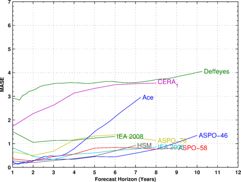
Fig. 5. – MASE values as a function of the forecast horizon. Year 1 is the baseline year when the forecast was issued.

Forecast	Date	2006	2008	2010	2013	2015	MASE2	Peak Date	Peak Value
All Liquids
Observed (All Liquids)		84.66	85.49	86.71	89.02	NA		2013-04	89.84
IEA (WEO)	2004	83.74	87.08	90.40	95.38	98.69	1.64	2030	121.30
IEA (WEO)	2005	85.85	89.35	92.50	96.62	99.11	2.33	2030	115.40
Koppelaar	2005	85.78	87.60	89.21	89.21	87.98	0.87	2011	89.58
Lahèrrere	2005	84.47	85.87	86.96	87.76	87.77	0.41	2014	87.84
EIA (IEO)	2006	84.50	88.23	91.60	95.76	98.30	2.09	2030	118.00
IEA (WEO)	2006	85.10	88.17	91.30	96.25	99.30	2.11	2030	116.30
CERA_1	2006	89.52	93.75	97.24	101.54	104.54	4.87	2035	130.00
Lahèrrere	2006	84.82	87.02	88.93	91.29	92.27	0.97	2018	92.99
Smith	2006	87.77	94.38	98.94	99.74	98.56	4.80	2012-05	99.83
IEA (WEO)	2008	83.15	85.51	88.15	92.13	94.40	0.94	2030	106.40
Crude Oil + NGL
Observed (EIA)		81.32	81.63	82.43	84.73	NA		2013-04	85.35
Ducan & Youngquist	1999	83.93	83.55	81.65	76.82	73.47	2.23	2007-01	83.95
Population based	2004	79.73	81.58	83.42	86.19	88.01	0.68	2050	110.64
GBM	2003	76.27	76.20	75.30	71.84	67.79	2.96	2007-05	76.34
Bakhtiari	2005	80.89	80.24	77.64	73.41	69.51	2.04	2006	80.89
ASPO-46	2004	80.95	80.59	80.00	77.13	73.77	1.11	2005	81.00
ASPO-58	2005	82.03	84.05	85.00	82.60	79.18	0.95	2010	85.00
Staniford (High)	2005	77.92	78.63	79.01	78.96	78.51	1.73	2011-10	79.08
Staniford (Med)	2005	75.94	75.91	75.52	74.27	73.00	3.23	2007-05	75.98
Staniford (Low)	2005	70.13	69.20	67.92	65.42	63.40	6.72	2002-07	70.88
IEA (WEO)	2006	81.38	83.96	86.50	90.26	92.50	1.76	2030	104.90
Smith	2006	82.81	88.27	91.95	90.97	88.60	3.50	2011-02	92.31
Loglets	2006	82.14	83.74	84.65	84.47	83.26	0.93	2012-01	84.80
ASPO-76	2006	79.00	85.06	90.00	87.72	85.00	2.26	2010	90.00
Robelius Low	2006	82.19	82.35	81.84	77.55	72.26	1.11	2007	82.50
Robelius High	2006	84.19	89.27	93.40	94.39	92.40	4.36	2012	94.54
Shock Model	2006	80.43	79.51	78.27	75.78	73.74	1.97	2003	81.17
EWG	2007	81.00	79.66	78.06	73.47	69.21	2.48	2005	81.76
IEA (WEO)	2008	79.80	81.59	83.40	85.97	87.40	0.56	2030	95.00
Crude Oil + Lease Condensate
Observed (EIA)		73.43	73.65	74.04	75.76	NA		2013-04	76.35
ASPO-46	2004	72.56	71.89	71.00	67.44	63.55	1.35	2005	72.80
Deffeyes	2004	66.07	65.83	65.30	63.96	62.73	4.06	2005-12	66.08
ASPO-58	2005	73.80	75.39	76.00	73.18	69.50	0.83	2010	76.00
IEA (WEO)	2006	71.78	73.76	75.70	78.60	80.30	0.85	2030	89.10
CERA_1	2006	76.89	80.35	82.29	83.18	83.83	3.56	2038	97.58
ASPO-76	2006	72.10	75.74	78.00	75.05	72.00	1.13	2010	78.00
HSM	2007	73.56	73.40	72.82	71.15	69.53	0.93	2006	73.56
Ace	2007	73.48	72.18	66.96	61.58	58.47	2.96	2006-01	73.55
IEA (WEO)	2008	69.73	70.64	71.46	72.49	73.00	1.31	2030	75.20

Table II. Summary of all the forecasts (figures are in mbpd) as well as the last EIA estimates.¹Productive capacities. ²MASE value for April 2013, the value in bold indicates the best forecast (i.e. the oldest with the lowest error).

Note the good performance of the population based model for crude oil and NGL (line in bold).

No peak oil?

Looking at crude oil + NGL production, we can consider two competitive models:

1. M0: The oil production will continue to grow with the world population at a constant rate of 4.3 barrels per capita per year (Figure 6).
2. M1: The production will fall according to the average peak oil forecast (Figure 7).

Fig 6.- Population based model (M0) for crude oil and NGL (C+C+NGL), the colored bands are 1-sigma, 1.5-sigma and 2-sigmas intervals (sigma= 1.25 million barrels per year).

Fig 7.- Average peak oil forecast (M1) for C+C+NGL calculated from 15 models that are predicting a peak before 2020 (Bakhtiari, Smith, Staniford, Loglets, Shock model, GBM, ASPO-[70,58,45], Robelius Low/High, HSM,Duncan&Youngquist). 95% of the predictions sees a production peak between 2008 and 2010 at 77.5 – 85.0 mbpd (The 95% forecast variability area in yellow is computed using a bootstrap technique). The magenta area is the 95% confidence interval for the population-based model. Click to Enlarge.
Regardless of economic parameters and the various peak oil scenarios, the M0 model has been an excellent predictor of the current supply levels  within a 1-sigma interval. We can then look at the probability that the observed production deviations are occuring by chance alone (which we note Prob(Deviation|M0)=p₀). It is clear that without  the addition of unconventional supply such as tar sands and tight oil we would have been much closer to the average peak oil scenario and close to a 2-sigmas deviation as illustrated on Figure 8 below.

A way to further stretch this analysis is to inject the knowledge of our average peak oil scenario M1 (Figure 7). Assuming that the “no peak oil” and “peak oil” events are equiprobable (uniform prior), we can then derive posterior probabilities from the Bayes rule:

Prob(M1 | Deviation) = Prob(Deviation | M1) / (Prob(Deviation | M0) + Prob(Deviation | M1))

Assuming our average peak oil scenario as M1, the probablity of this scenario is now around 1%, excluding unconventional sources we get to 15% (no tight oil) and 70% (no Canadian Tar Sands).

Fig 9.- Posterior probability values for a peak oil event for C+C+NGL.

Supply and Demand Equilibrium

Supply is just one part of the equation. Demand is even harder to predict and highly volatile. Since 2005, global fuel consumption has strongly deviated from nominal levels by almost 10 million barrels per day due to the persistent high price environment and lower economic output.

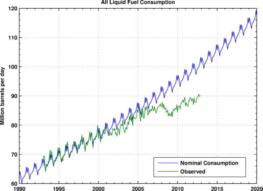
Fig 11.- Observed total liquid fuel consumption (EIA data) and nominal consumption level based on 1993-2001 period.

Since the 2009 financial crisis, growth in advanced economies has been weak. Recovery from the great recession is still ongoing and has been exceptionally long:

Fig 11.- US GDP cyclical component (src).

In their last economic outlook update, the IMF is forecasting just 3% growth for the world GDP.

In chapter 3 of the April 2011 IMF World Economic Outlook, the IMF economists derived short term income elasticity of energy demand values between 0.47 and 0.83 (high price environment) which means that a 1% rise in  income (global GDP) can lead to an increase in oil demand between 0.5 and 1.0%. Therefore, given the current global growth forecast, oil supply growth (all liquids) should be above 2% a year and we are struggling to maintain a 1% growth.

Fig 12.- Expected oil demand growth rates based on the IMF data. The observed supply growth rate (all liquids) is a year-on-year growth rate after a 12 months moving average.
 

Final Thoughts

 

 

• Econ 101 works. High oil prices reduce consumption and increase marginal supply, however, with vastly different short term and long term price elasticity values.
• Most peak oil forecasts can be dismissed but none of them could have factored in contributions from marginal unconventional sources such as shale oil.
• We will see a second production peak for OECD countries of unknown duration (see chart above).
• Unconventional marginal oil supply sources have saved the day for now, however, double digit growth in tight oil production could also mean double digit decline.
• No one knows how long the tight oil boom will last or how it will spread to the rest of the world, so we are still in the dark. Forecasting future production capacity is more uncertain and difficult than ever as we cannot just track a set of Tier one giant fields. Unconventional and marginal sources of supply are now making a difference and are more scattered and difficult to track.
• Despite large investments, exceptional exploration efforts and widespread application of enhanced oil recovery techniques (EOR), supply from conventional oil has been flat since 2005 and has probably peaked (so Kenneth Deffeyes was not completely wrong).
• Peak demand? maybe, but what about peak GDP growth? there is still and output gap between actual GDP and potential GDP.
• Prices are likely to stay elevated and volatile as demand periodically hits its head on a tight supply ceiling and will continue to depress demand (others would say destroy) and constrain growth rates. On the flip side, it will help spur efficiency gains, innovation, production from marginal source of supply, alternative transportation modes, etc.

Ref:

[1] Rob J. Hyndman, Anne B. Koehler, Another look at measures of forecast accuracy, International Journal of Forecasting, Volume 22, Issue 4, October-December 2006, Pages 679-688. pdf available here.
[1] Helbling, T., Kang, J.S., Kumhof, M., Muir, D., Pescatori, A. and Roache, S. (2011), “Oil Scarcity, Growth, and Global Imbalances”, World Economic Outlook, April 2011, Chapter 3, International Monetary Fund.

Thank You!

Ok, enough with the psychedelic charting, I would like to express my gratitude to the founders of this one of a kind website (Prof. Goose and HO) as well as all the staff, contributors and all the TODers. They did a tremendous service to society by raising energy awareness, all of that as volunteers on their free time. I joined this site back in 2004 at the time peak oil was a fringe topic struggling to keep its spot between big foot and UFOs. At that time, I was completely energy illiterate and this forum opened my eyes on one of the most complex issue facing our modern world. Ultimately, it completely changed my views on our future on this planet. After 8 years, I can appreciate the ground covered since as peak oil is now routinely debated in mainstream media. TOD was never about being right or wrong on the exact timing or shape of peak oil. TOD is a wakeup call on our energy predicament. Modern civilization was built upon cheap fossil fuel and it may cause its downfall. Finally, I urge decision makers not to turn their back on energy issues. TOD is going away but not resource depletion. If I learned one thing during this journey is that we cannot be reactive on these kinds of complex issues, we must be proactive. Our dependence on fossil fuels is as strong as ever and humanity faces tremendous challenges this century especially when considering potential impacts from climate change.

Thank you and good luck to all, I’ll try to post periodically on my personal blog if you want to keep in touch with me.

the oil drum

4 Comments on "Peak Oil Update – Final Thought"

Arthur on Mon, 19th Aug 2013 1:06 pm 



“I urge decision makers not to turn their back on energy issues.”

This suggests that policy makers actually can afford to ignore energy issues for a long time to come. What does TOD know that we don’t?

“TOD was never about being right or wrong on the exact timing or shape of peak oil.”

This can be interpreted as TOD admitting that in fact peak fossil is further away in time than previously thought by many TOD-lers.

“Most peak oil forecasts can be dismissed but none of them could have factored in contributions from marginal unconventional sources such as shale oil.”

Sounds like an excuse.

“Prices are likely to stay elevated and volatile as demand periodically hits its head on a tight supply ceiling and will continue to depress demand (others would say destroy) and constrain growth rates. On the flip side, it will help spur efficiency gains, innovation, production from marginal source of supply, alternative transportation modes, etc.”

Amen. The new development is more or less a Godsend (excluding environmental issues, but including dieoff avoidance), providing a non-catastrophic path into the ‘renewable energy nirwana’.

Jerry McManus on Mon, 19th Aug 2013 4:49 pm 



Another myopic, misleading, and ultimately pointless “analysis” from the eggheads at TOD.

All the Hubbert model really says is that the area under the production curve will eventually equal the area under the discovery curve. Hubbert NEVER made any “predictions” about the shape of either curve.

Furthermore, the most salient fact in this article is the demand destruction:

“global fuel consumption has strongly deviated from nominal levels by almost 10 million barrels per day due to the persistent high price environment and lower economic output.”

That is entirely consistent with the analysis done 40 years ago by the authors of the “Limits to Growth” report which shows resource constraints sapping so much capital from the rest of the economy that it leads to a non-linear response in the form of a collapse in the first decades of the 21st century.

Don’t bother trying to point that out to the pointy heads at TOD, they will simply sneer something about “doomers” and go back to their pointless bean counting.

Sparky on Tue, 20th Aug 2013 1:39 am 



.
Thanks for the psychedelic charts ,
I’m not so sure if the ratio per person is appropriate without some correction factor , the bottom half of the world population is not consuming much even though their (small )consumption has been rising faster .

As a rough and ready index of peak oil , I watche the airline industry
it is totally dependent on high quality distillates ,
there is not much efficiency to be gained
it is very market driven

My chosen guide for the peak is Lahèrrere ,
his forecasts have always been spot on , consistently

Harquebus on Tue, 20th Aug 2013 4:52 am 



He forgets. The increase in oil production was paid for on credit. The world can not afford triple digit barrels and pay off debt.